How to use ajustador to fit a moose_nerp model
An optimization procedure consists of the following “components”:
The short version is:
>>> import measurements1
>>> import ajustador as aju
>>> exp_to_fit = measurements1.waves042811[[0, 6, 23]]
>>> params = aju.optimize.ParamSet(
... ('RA',           4.309,  0,   100),
... ('RM',           0.722,  0,    10),
... ('CM',           0.015,  0, 0.100))
>>> fitness = aju.fitnesses.combined_fitness()
>>> fit = aju.optimize.Fit('quick-start-d1.fit',
...                        exp_to_fit,
...                        'd1d2', 'D1',
...                        fitness,
...                        params)
>>> fit.do_fit(15, popsize=5)                          # DOCTEST: +SKIP
>>> fit.param_names()
['RA', 'RM', 'CM']
>>> fit.params.unscale(fit.optimizer.result()[0])  # parameters
[1.6781569599861799, 4.4270115380320281, 0.02983857703183539]
>>> fit.params.unscale(fit.optimizer.result()[6])  # stddevs
[0.7099180820095562, 0.73484996358979826, 0.0033816805879411456]
The long version is below.
Experimental recording
An “experiment” is described by a ajustador.loader.Measurement object.
As an example, let’s use measurements1.042811, a current-clamp
recording from a striatal D1 neuron:
>>> import measurements1
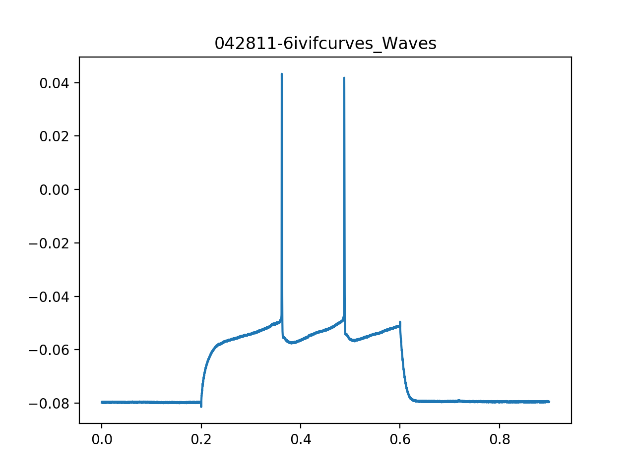
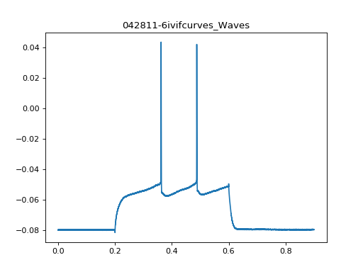
>>> exp = measurements1.waves042811
>>> exp.name
'042811-6ivifcurves_Waves'
The data is stored in the .waves attribute:
>>> type(exp.waves), len(exp.waves)
(<class 'numpy.ndarray'>, 24)
Each “wave” is a single measurement, a subclass of ajustador.loader.Trace.
It has a bunch of attributes like injection voltage:
>>> exp.waves[0]
<ajustador.loader.IVCurve object at 0x7f691bd63198>
>>> exp.waves[0].injection
-5e-10
The actual data is in .wave attribute:
>>> exp.waves[22].wave.x
array([  0.00000000e+00,   1.00000000e-04,   2.00000000e-04, ...,
         8.99700000e-01,   8.99800000e-01,   8.99900000e-01])
>>> exp.waves[22].wave.y
array([-0.0798125 , -0.07953125, -0.0795    , ..., -0.07959375,
       -0.079625  , -0.07953125], dtype=float32)
(Source code, png, hires.png, pdf)
Simulated model
The model that matches our experimental data is the d1d2 model of D1 and D2 striatal neurons using MOOSE:
>>> from moose_nerp import d1d2
>>> d1d2.param_cond.Condset.D1
D1(Krp={(0, 2.61e-05): 150.963, (2.61e-05, 5e-05): 70.25, (5e-05, 0.001): 77.25},
   KaF={(0, 2.61e-05): 600, (2.61e-05, 5e-05): 500, (5e-05, 0.001): 100},
   KaS={(0, 2.61e-05): 404.7, (2.61e-05, 5e-05): 35.2, (5e-05, 0.001): 0},
   Kir={(0, 2.61e-05): 9.4644, (2.61e-05, 5e-05): 9.4644, (5e-05, 0.001): 9.4644},
   CaL13={(0, 2.61e-05): 12, (2.61e-05, 5e-05): 5.6, (5e-05, 0.001): 5.6},
   CaL12={(0, 2.61e-05): 8, (2.61e-05, 5e-05): 4, (5e-05, 0.001): 4},
   CaR={(0, 2.61e-05): 20, (2.61e-05, 5e-05): 45, (5e-05, 0.001): 44},
   CaN={(0, 2.61e-05): 4.0, (2.61e-05, 5e-05): 0.0, (5e-05, 0.001): 0.0},
   CaT={(0, 2.61e-05): 0.0, (2.61e-05, 5e-05): 1.9, (5e-05, 0.001): 1.9},
   NaF={(0, 2.61e-05): 130000.0, (2.61e-05, 5e-05): 1894, (5e-05, 0.001): 927},
   SKCa={(0, 2.61e-05): 0.5, (2.61e-05, 5e-05): 0.5, (5e-05, 0.001): 0.5},
   BKCa={(0, 2.61e-05): 10.32, (2.61e-05, 5e-05): 10, (5e-05, 0.001): 10})
The most convenient way to run the simulation is through the optimization object, so we’ll do that in on of the later subsections.
Feature functions
The :module:`ajustador.features` module contains a bunch of “feature functions” which attempt to extract interesting characteristics from the experimental and simulated traces.
>>> import ajustador as aju
>>> pprint.pprint(aju.features.Spikes.provides)
('spike_i',
 'spikes',
 'spike_count',
 'spike_threshold',
 'mean_isi',
 'isi_spread',
 'spike_latency',
 'spike_bounds',
 'spike_height',
 'spike_width',
 'mean_spike_height')
Before using those autodetected functions it is prudent to check that they work as expected for the data in question. Oftentimes this is not the case, and it is necessary to adjust the functions or some parameters to achieve proper behaviour.
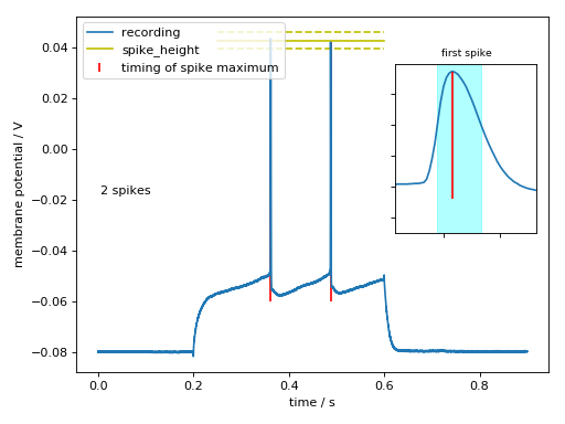
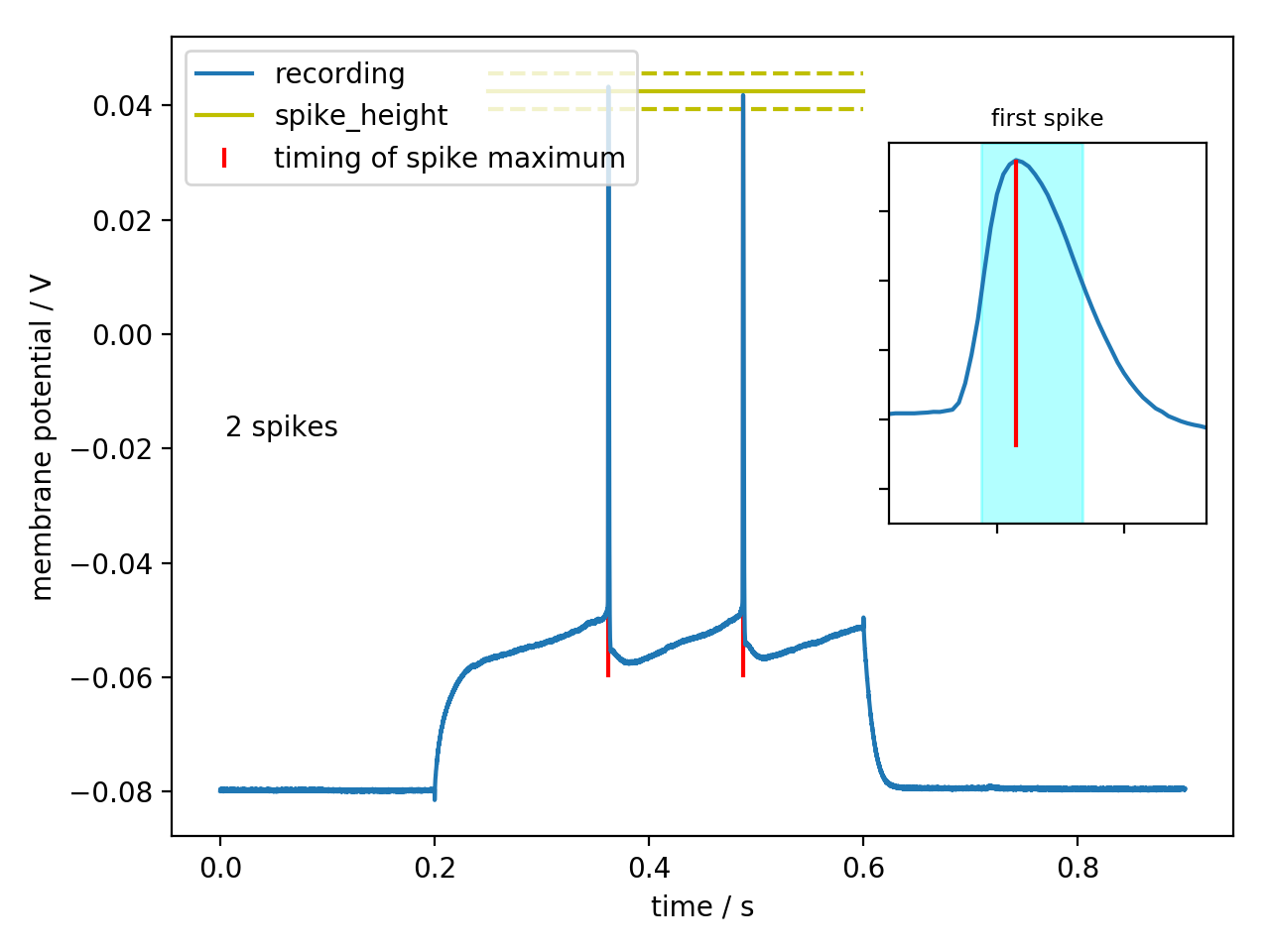
Each ajustador.features.Feature object has a way to present
the extracted values in both graphical and textual modes:
>>> aju.features.Spikes(exp.waves[22]).plot()
(Source code, png, hires.png, pdf)

>>> print(aju.features.Spikes(exp.waves[22]).report())
spike_i = 7243
          9755
spikes = (0.36215, 0.04331250116229057)
         (0.48775, 0.04184374958276749)
spike_count = 2
spike_threshold = -0.047031249851
                  -0.0484062507749
                = -0.0477±0.0010
mean_isi = 0.126±0.001
isi_spread = nan
spike_latency = 0.16215
spike_bounds = WaveRegion[16 points, x=0.3619-0.3627, y=0.002-0.043]
               WaveRegion[17 points, x=0.4875-0.4883, y=-0.000-0.042]
spike_height = 0.0903437510133
               0.0902500003576
             = 0.09030±0.00007
spike_width = 0.0008
              0.00085
            = 0.00082±0.00004
mean_spike_height = 0.043±0.001
For a list of the provided feature functions, refer to the ajustador.features module docs.
Fitness functions
In a normal fit, we wan to combine multiple fitness functions to
achieve fit that optimizes multiple characteristics. The
ajustador.fitnesses.combined_fitness class does that.
Since we don’t have any experimental data yet, we’ll just
“test” how close are two experimental measurements (for different
cells of the same type):
>>> exp2 = measurements1.waves050511
>>> fitness = aju.fitnesses.combined_fitness()
>>> fitness(exp, exp2)
0.49338569891028333
>>> print(fitness.report(exp, exp2))
response_fitness=1*0.7=0.7
baseline_pre_fitness=1*0.0039=0.0039
baseline_post_fitness=1*0.0029=0.0029
rectification_fitness=1*0.64=0.64
falling_curve_time_fitness=1*0.12=0.12
spike_time_fitness=1*0.17=0.17
spike_width_fitness=1*0.3=0.3
spike_height_fitness=1*0.031=0.031
spike_latency_fitness=1*0.75=0.75
spike_ahp_fitness=1*0.072=0.072
ahp_curve_fitness=1*0.96=0.96
spike_range_y_histogram_fitness=1*0.63=0.63
total: 0.49
As we can see, some measures like baseline are very close, spike timing and AHPs depth are quite similar, but AHP shape and the passive parameters (“rectification”) are futher apart.
If one of those is replaced with a model, the optimization will
try to decrease the total value which is a weighted average of the
fitness functions. It is possible to override the weights of
component fitness functions, as well as to add new fitness functions
to the mix. Refer to the ajustador.fitnesses.combined_fitness
class documentation for more details.
Simulation and optimization loop
When fitting the model to experimental data, we recreate the
experimental procedure during simulation. Currently only a rectangular
injection is supported. It is described by the
ajustador.loader.Trace objects:
>>> exp[0].injection_start
0.2
>>> exp[0].injection_end
0.6
>>> exp[0].injection
-5e-10
We could simulate for all injection values, but the results
wouldn’t be significantly better then if we just fit for a few
“representative” values. We can pick the highest hyperpolarizing
injection, a small hyperpolarizing injection, and one where
spiking occurs:
>>> exp.injection * 1e12      # convert from A to pA
array([-500., -450., -400., -350., -300., -250., -200., -150., -100.,
        -50.,    0.,   50.,  100.,  150.,  200.,  200.,  220.,  240.,
        260.,  280.,  300.,  320.,  340.,  360.])
>>> import numpy as np
>>> np.arange(len(exp))[exp.injection < 0]
array([0, 1, 2, 3, 4, 5, 6, 7, 8, 9])
>>> np.arange(len(exp))[exp.spike_count > 0]
array([22, 23])
The ajustador.loader.Measurement class is designed
to behave a bit like a numpy.ndarray, and operations
like simple and fancy indexing are supported. We make use of this
to pick out traces 0, 6, and 23 by indexing with a list:
>>> exp_to_fit = exp[[0, 6, 23]]
In the optimization loop, the ajustador.optimize.Optimizer
class is used as a wrapper for the actual fitting algorithm. We
need to specify which parameters are allowed to vary, and
within what ranges [1].
To make things simple, we’ll fit the passive electrical characteristics of the membrane \(R_\text{m}\), \(C_\text{m}\), and \(R_\text{a}\):
>>> params = aju.optimize.ParamSet(
... # (name,starting value, lower bound, upper bound)
... ('RA',           4.309,  0,   100),
... ('RM',           0.722,  0,    10),
... ('CM',           0.015,  0, 0.100))
The precise values of the bounds are not important — ideally the optimum parameters will be clustered away from either of the bounds.
The optimization object uses the experimental traces, fitness function, and parameter set created above. We also need to specify that we’ll be using the d1d2 model and its D1 neuron. Simulation results (voltage traces from the soma) are stored in the directory specified as the first argument:
>>> fit = aju.optimize.Fit('quick-start-d1.fit',
...                        exp_to_fit,
...                        'd1d2', 'D1',
...                        fitness,
...                        params)
After this lengthy preparation, we are now ready to perform some actual fitting:
>>> fit.do_fit(15, popsize=5) # DOCTEST: +SKIP
This will perform \(15 \times 5 \times 3 = 225\) simulations, hopefully moving in the direction of better parameters [2]. Individual simulations are executed in parallel, so it’s best to run this on a multi-core machine.
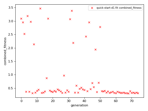
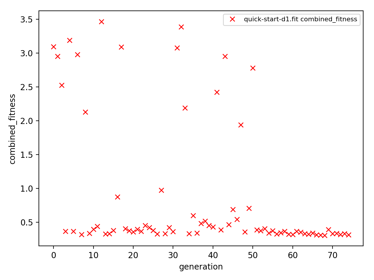
We can visualize the convergence of the fit by plotting
the fitness score of each of the simulation points. (That’s
\(15 \times 5 = 75\) points, because we get a single score
for each of the three simulations recreating our “experiment”
exp_to_fit.)
We need to import :module:`ajustador.drawing` separately.
>>> import ajustador.drawing
>>> aju.drawing.plot_history(fit, fit.measurement)
(Source code, png, hires.png, pdf)

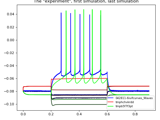
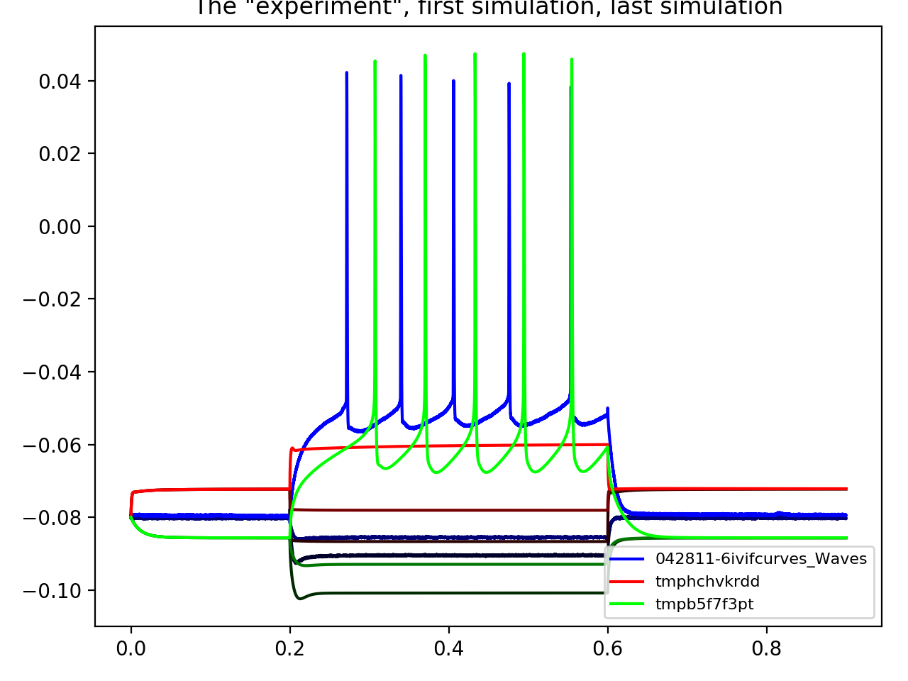
When clicking on the points on this graph, a new window will be opened showing the experimental and simulated traces. We can always plot some set traces explicitly:
>>> aju.drawing.plot_together(fit.measurement, fit[0], fit[-1]) # DOCTEST: +SKIP
(Source code, png, hires.png, pdf)

Usually we care about the numerical result. The result of CMA are are a “center” value and the estimate of standard deviations of each parameter:
>>> fit.param_names()
['RA', 'RM', 'CM']
>>> fit.params.unscale(fit.optimizer.result()[0])
[1.6781569599861799, 4.4270115380320281, 0.02983857703183539]
>>> fit.params.unscale(fit.optimizer.result()[6])
[0.7099180820095562, 0.73484996358979826, 0.0033816805879411456]
This does not correspond to any specific simulation, but is the best estimate based on the history of optimization. The simulations in the tail of the optimization are drawn from this distribution.
If we let the optimization run for a longer time, we would hope for a better fit. We can expect the optimization to stop making noticable progress after about 1000 points.
| [1] | The algorithm does not know what are the physiologically sensible ranges of parameters. If e.g. a negative resistivity is selected, most likely the resulting simulation will not resemble a the experimental recording and will be rejected, but this is a very inefficient way to reject infeasible parameter values. |
| [2] | Notionally, the optimization loop has a stop condition, but it’s very very unlikely that we’ll hit it within a couple hundred steps. |