ajustador.features¶

SteadyState¶

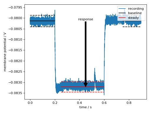
class ajustador.features.SteadyState(obj)[source]¶

Find the baseline and injection steady states

The range before baseline_before and after baseline_after is used for baseline.

The range between steady_after and steady_before is used for steady.

>>> import measurements1
>>> import ajustador

>>> rec = measurements1.waves042811[8]
>>> feat = ajustador.features.SteadyState(rec)
>>> print(feat.report())
baseline = -0.08014±0.00002
steady = -0.08320±0.00009
response = -0.00306±0.00009
baseline_pre = -0.08015±0.00003
baseline_post = -0.08011±0.00004

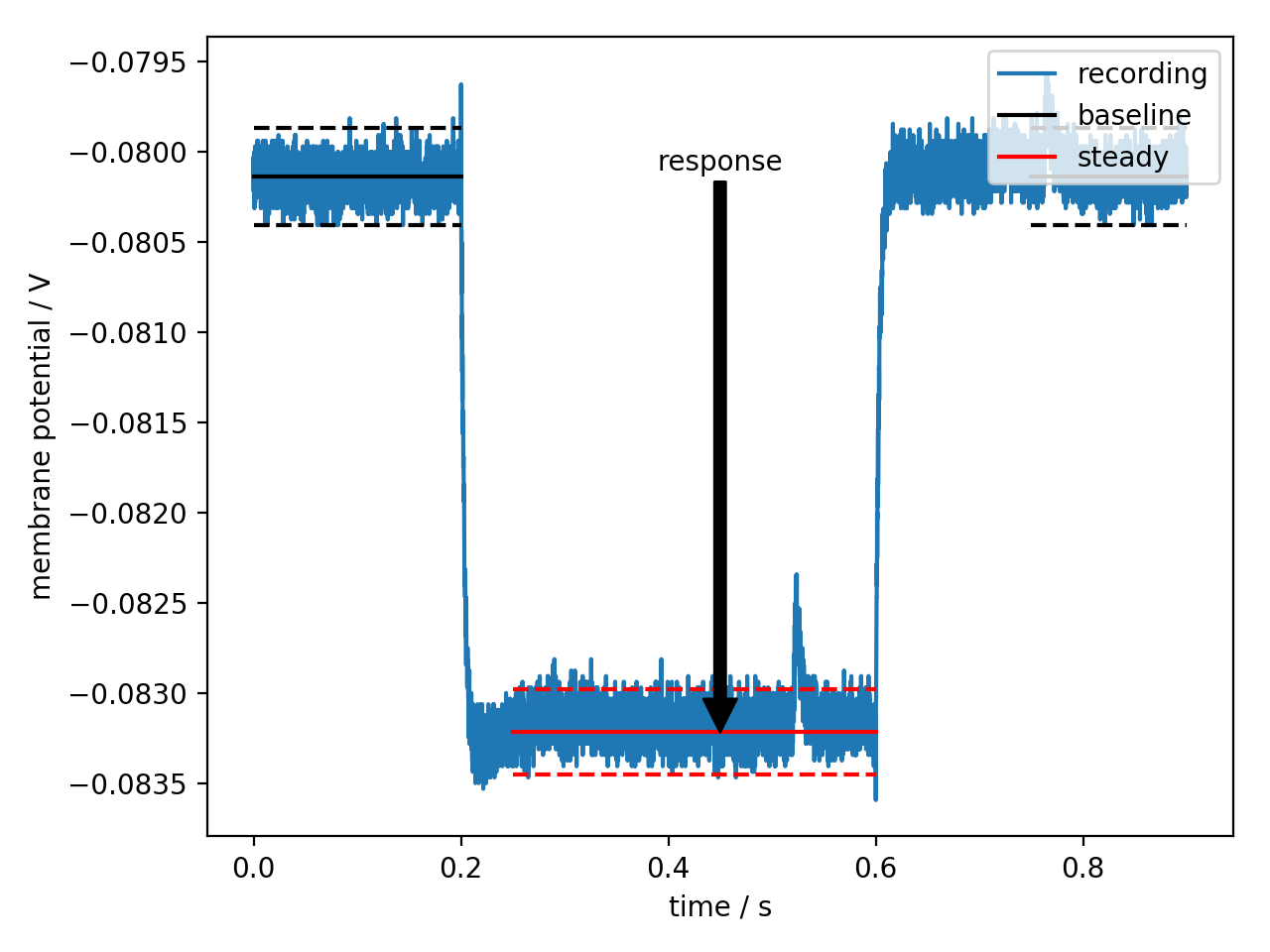
(Source code, png, hires.png, pdf)

>>> rec = strange1.high_baseline_post[-1]
>>> feat = ajustador.features.SteadyState(rec)
>>> print(feat.report())
baseline = -0.07±0.02
steady = -0.04±0.02
response = 0.03±0.03
baseline_pre = -0.078265±0.000002
baseline_post = -0.01533±0.00006

Additional plots for SteadyState

requires = ('wave', 'baseline_before', 'baseline_after', 'steady_after', 'steady_before', 'steady_cutoff')¶

provides = ('baseline', 'steady', 'response', 'baseline_pre', 'baseline_post')¶

mean_attributes = ('baseline', 'steady', 'response', 'baseline_pre', 'baseline_post')¶

array_attributes = ('baseline', 'steady', 'response', 'baseline_pre', 'baseline_post')¶

baseline¶

The mean voltage of the area outside of injection interval

Returns mean value of wave after excluding “outliers”, values > 95th or < 5th percentile.

baseline_pre¶

The mean voltage of the area before the injection interval

Returns mean value of wave after excluding “outliers”, values > 95th or < 5th percentile.

baseline_post¶

The mean voltage of the area after the injection interval

Returns mean value of wave after excluding “outliers”, values > 95th or < 5th percentile.

steady¶

Returns mean value of wave between steady_after and steady_before.

“Outliers”, values > 80th percentile (which is a parameter), are excluded. 80th percentile excludes the spikes.

response¶

plot(figure=None, pre_post=False)[source]¶

Spikes¶

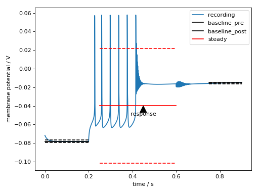
class ajustador.features.Spikes(obj)[source]¶

Find the position and height of spikes

(Source code, png, hires.png, pdf)

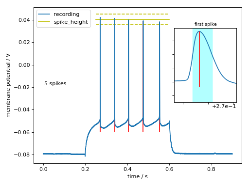
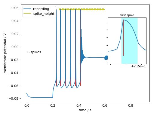
>>> rec = measurements1.waves042811[-1]
>>> feat = ajustador.features.Spikes(rec)
>>> print(feat.report())
spike_i = 5433
          6795
          8121
          9518
          11077
spikes = (0.27165, 0.042249999940395355)
         (0.33975, 0.04143749922513962)
         (0.40605, 0.040031250566244125)
         (0.47590000000000005, 0.039281249046325684)
         (0.5538500000000001, 0.038343749940395355)
spike_count = 5
spike_threshold = -0.0497187487781
                  -0.047187499702
                  -0.046250000596
                  -0.0472187511623
                  -0.0475312508643
                = -0.048±0.001
mean_isi = 0.071±0.005
isi_spread = 0.01165
spike_latency = 0.07165
spike_bounds = WaveRegion[16 points, x=0.2714-0.2722, y=0.001-0.042]
               WaveRegion[16 points, x=0.3395-0.3403, y=0.001-0.041]
               WaveRegion[16 points, x=0.4058-0.4066, y=0.000-0.040]
               WaveRegion[17 points, x=0.4756-0.4765, y=-0.002-0.039]
               WaveRegion[17 points, x=0.5536-0.5544, y=-0.004-0.038]
spike_height = 0.0919687487185
               0.0886249989271
               0.0862812511623
               0.0865000002086
               0.0858750008047
             = 0.088±0.003
spike_width = 0.0008
              0.0008
              0.0008
              0.00085
              0.00085
            = 0.00082±0.00003
mean_spike_height = 0.040±0.002

(Source code, png, hires.png, pdf)

>>> rec = strange1.high_baseline_post[-1]
>>> feat = ajustador.features.Spikes(rec)
>>> print(feat.report())
spike_i = 1139
          1298
          1491
          1686
          1881
          2078
spikes = (0.22782531673705267, 0.057194696302130574)
         (0.2596288508557457, 0.05766577375785903)
         (0.2982331406979329, 0.05768073942459968)
         (0.33723747499444323, 0.05737642815217372)
         (0.3762418092909535, 0.0578476478258447)
         (0.41564618804178705, 0.05776826735137781)
spike_count = 6
spike_threshold = -0.0434335444769
                  -0.0422116029017
                  -0.0418710702884
                  -0.0406300647089
                  -0.0425443984716
                  -0.0418791194138
                = -0.0421±0.0009
mean_isi = 0.038±0.003
isi_spread = 0.00760084463214
spike_latency = 0.0278253167371
spike_bounds = WaveRegion[5 points, x=0.2277-0.2287, y=0.008-0.057]
               WaveRegion[5 points, x=0.2595-0.2605, y=0.024-0.058]
               WaveRegion[5 points, x=0.2981-0.2991, y=0.025-0.058]
               WaveRegion[6 points, x=0.3369-0.3381, y=0.019-0.057]
               WaveRegion[6 points, x=0.3761-0.3773, y=0.013-0.058]
               WaveRegion[6 points, x=0.4155-0.4167, y=0.008-0.058]
spike_height = 0.100628240779
               0.0998773766596
               0.099551809713
               0.0980064928611
               0.100392046297
               0.0996473867652
             = 0.0997±0.0009
spike_width = 0.00100011113581
              0.00100011113581
              0.00100011113581
              0.00120013336297
              0.00120013336297
              0.00120013336297
            = 0.0011±0.0001
mean_spike_height = 0.0576±0.0003

Additional plots for Spikes

requires = ('wave', 'injection_interval', 'injection_start')¶

provides = ('spike_i', 'spikes', 'spike_count', 'spike_threshold', 'mean_isi', 'isi_spread', 'spike_latency', 'spike_bounds', 'spike_height', 'spike_width', 'mean_spike_height')¶

array_attributes = ('spike_count', 'spike_height', 'spike_width', 'mean_isi', 'isi_spread', 'spike_latency')¶

mean_attributes = ('spike_height', 'spike_width', 'spike_threshold')¶

spike_i_and_threshold¶: Indices of spike maximums in the wave.x, wave.y arrays

spike_i¶: Indices of spike maximums in the wave.x, wave.y arrays

spike_threshold¶: Indices of spike maximums in the wave.x, wave.y arrays

spikes¶: An array with .x and .y components marking the spike maximums

spike_count¶: The number of spikes

mean_isi_fallback_variance = 0.001¶

mean_isi¶

The mean interval between spikes

Defined as:

\(<x_{i+1} - x_i>\), if there are at least two spikes,
the length of the depolarization interval otherwise (injection_interval)

If there less than three spikes, the variance is fixed as mean_isi_fallback_variance.

isi_spread¶

The difference between the largest and smallest inter-spike intervals

Only defined when spike_count is at least 3.

spike_latency¶: Latency until the first spike or nan if no spikes

spike_bounds¶: The FWHM box and other measurements for each spike

spike_height¶: The difference between spike peaks and spike threshold

spike_width¶

mean_spike_height¶: The mean absolute position of spike vertices

plot(figure=None)[source]¶

spike_plot(figure=None, **kwargs)[source]¶

AHP¶

class ajustador.features.AHP(obj)[source]¶

Find the depth of “after hyperpolarization”

(Source code, png, hires.png, pdf)

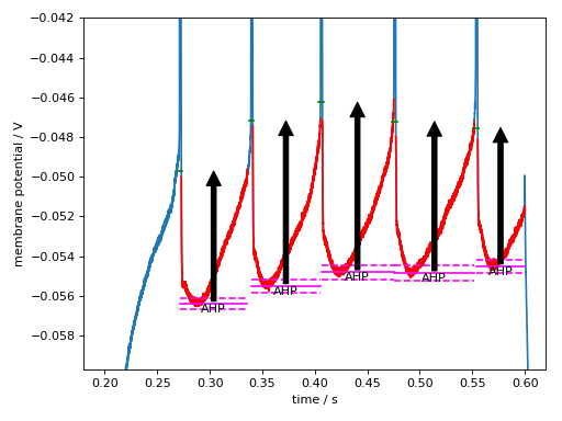
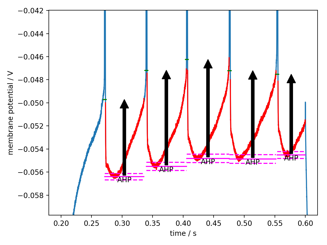
>>> rec = measurements1.waves042811[-1]
>>> feat = ajustador.features.AHP(rec)
>>> print(feat.report())
spike_ahp_window = WaveRegion[1259 points, x=0.2729-0.3358, y=-0.057--0.050]
                   WaveRegion[1287 points, x=0.3409-0.4053, y=-0.056--0.047]
                   WaveRegion[1360 points, x=0.4073-0.4753, y=-0.055--0.046]
                   WaveRegion[1496 points, x=0.4772-0.5520, y=-0.055--0.047]
                   WaveRegion[896 points, x=0.5552-0.6000, y=-0.055--0.048]
spike_ahp = -0.05640±0.00009
            -0.05551±0.00012
            -0.05481±0.00012
            -0.05487±0.00013
            -0.05452±0.00010
          = -0.05533±0.00005
spike_ahp_position = 0.2864±0.0002
                     0.3561±0.0002
                     0.4224±0.0002
                     0.4910±0.0002
                     0.5680±0.0003

requires = ('wave', 'injection_start', 'injection_end', 'injection_interval', 'spikes', 'spike_count', 'spike_bounds', 'spike_threshold')¶

provides = ('spike_ahp_window', 'spike_ahp', 'spike_ahp_position')¶

array_attributes = ('spike_ahp_window', 'spike_ahp', 'spike_ahp_position')¶

mean_attributes = ('spike_ahp',)¶

spike_ahp_window¶

spike_ahp¶

Returns the (averaged) minimum in y of each AHP window

spike_ahp_window is used to determine the extent of the AHP. An average of the bottom area of the window of the width of the spike is used.

spike_ahp_position¶

Returns the (averaged) x of the minimum in y of each AHP window

spike_ahp_window is used to determine the extent of the AHP. An average of the bottom area of the window of the width of the spike is used.

TODO: add to plot

plot(figure=None)[source]¶

spike_plot(figure=None, **kwargs)[source]¶

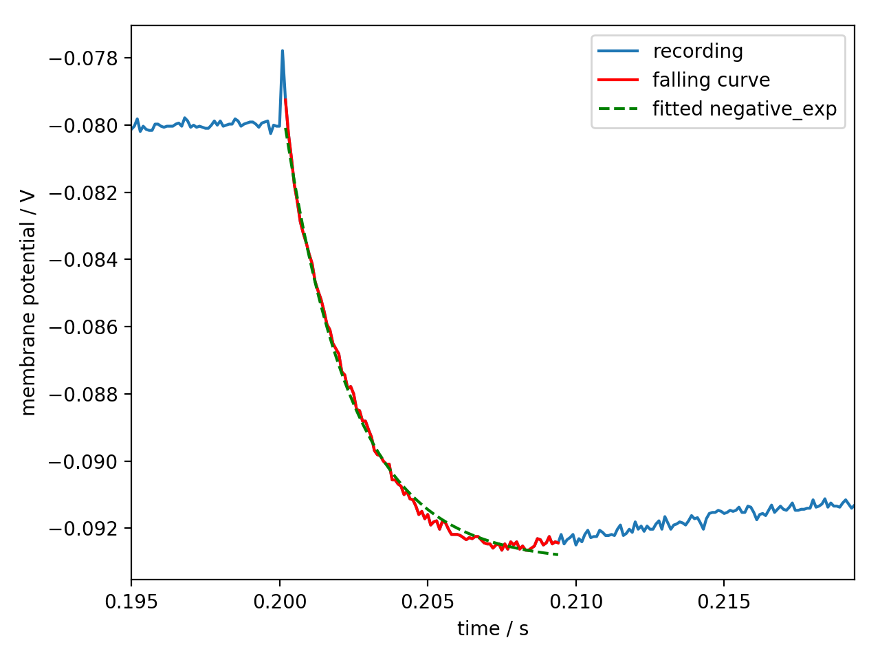
FallingCurve¶

class ajustador.features.FallingCurve(obj)[source]¶

(Source code, png, hires.png, pdf)

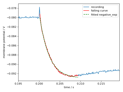
>>> rec = measurements1.waves042811[0]
>>> feat = ajustador.features.FallingCurve(rec)
>>> print(feat.report())
falling_curve = (0.2001, -0.07778125256299973)
                (0.20020000000000002, -0.07925000041723251)
                (0.2003, -0.08025000244379044)
                (0.20040000000000002, -0.08096875250339508)
                (0.2005, -0.08178125321865082)
                (0.2006, -0.08228124678134918)
                (0.20070000000000002, -0.08287499845027924)
                (0.2008, -0.08321875333786011)
                (0.20090000000000002, -0.08349999785423279)
                (0.201, -0.08384375274181366)
                (0.2011, -0.08412499725818634)
                (0.20120000000000002, -0.0846562534570694)
                (0.2013, -0.08493749797344208)
                (0.20140000000000002, -0.08518750220537186)
                (0.2015, -0.08553124964237213)
                (0.2016, -0.0859375)
                (0.20170000000000002, -0.08609375357627869)
                (0.2018, -0.08649999648332596)
                (0.2019, -0.08665625005960464)
                (0.202, -0.08681250363588333)
                (0.2021, -0.08734375238418579)
                (0.20220000000000002, -0.08743750303983688)
                (0.2023, -0.08784375339746475)
                (0.2024, -0.08778125047683716)
                (0.2025, -0.08799999952316284)
                (0.2026, -0.0884687528014183)
                (0.20270000000000002, -0.0885000005364418)
                (0.2028, -0.08881250023841858)
                (0.2029, -0.08881250023841858)
                (0.203, -0.08906249701976776)
                (0.2031, -0.08928125351667404)
                (0.20320000000000002, -0.08968749642372131)
                (0.2033, -0.0898125022649765)
                (0.2034, -0.08984375)
                (0.20350000000000001, -0.09000000357627869)
                (0.2036, -0.09009374678134918)
                (0.20370000000000002, -0.09009374678134918)
                (0.2038, -0.09056250005960464)
                (0.2039, -0.09056250005960464)
                (0.20400000000000001, -0.09068749845027924)
                (0.2041, -0.09075000137090683)
                (0.20420000000000002, -0.09099999815225601)
                (0.2043, -0.09090624749660492)
                (0.2044, -0.0911249965429306)
                (0.20450000000000002, -0.0911562517285347)
                (0.2046, -0.09134375303983688)
                (0.20470000000000002, -0.09159374982118607)
                (0.2048, -0.09149999916553497)
                (0.2049, -0.09171874821186066)
                (0.20500000000000002, -0.09159374982118607)
                (0.2051, -0.09190624952316284)
                (0.20520000000000002, -0.09181249886751175)
                (0.2053, -0.09178125113248825)
                (0.2054, -0.09203124791383743)
                (0.20550000000000002, -0.09178125113248825)
                (0.2056, -0.09184374660253525)
                (0.20570000000000002, -0.09203124791383743)
                (0.2058, -0.09218750149011612)
                (0.2059, -0.09218750149011612)
                (0.20600000000000002, -0.09218750149011612)
                (0.2061, -0.09221874922513962)
                (0.20620000000000002, -0.09228125214576721)
                (0.2063, -0.09234374761581421)
                (0.2064, -0.09228125214576721)
                (0.20650000000000002, -0.09231249988079071)
                (0.2066, -0.09224999696016312)
                (0.20670000000000002, -0.09224999696016312)
                (0.2068, -0.09234374761581421)
                (0.2069, -0.0924374982714653)
                (0.20700000000000002, -0.0924687534570694)
                (0.2071, -0.0924687534570694)
                (0.20720000000000002, -0.09259375184774399)
                (0.2073, -0.0925000011920929)
                (0.2074, -0.0924687534570694)
                (0.20750000000000002, -0.09265624731779099)
                (0.2076, -0.0924687534570694)
                (0.20770000000000002, -0.09262499958276749)
                (0.2078, -0.0924062505364418)
                (0.2079, -0.0925000011920929)
                (0.20800000000000002, -0.0924062505364418)
                (0.2081, -0.09262499958276749)
                (0.2082, -0.0925312489271164)
                (0.2083, -0.09265624731779099)
                (0.2084, -0.09265624731779099)
                (0.20850000000000002, -0.09259375184774399)
                (0.2086, -0.0925312489271164)
falling_curve_fit = <function negative_exp at 0x7f79d20816a8>
                    falling_param(amp=vartype(-0.01329, 0.00011), tau=vartype(0.002524, 0.000058))
                    True
falling_curve_amp = -0.0133±0.0001
falling_curve_tau = 0.00252±0.00006
falling_curve_function = <function negative_exp at 0x7f79d20816a8>

Additional plots for FallingCurve

requires = ('wave', 'injection_start', 'steady_before', 'falling_curve_window', 'baseline', 'steady')¶

provides = ('falling_curve', 'falling_curve_fit', 'falling_curve_amp', 'falling_curve_tau', 'falling_curve_function')¶

array_attributes = ('falling_curve_amp', 'falling_curve_tau', 'falling_curve_function')¶

falling_curve¶

falling_curve_fit¶

falling_curve_amp¶

falling_curve_tau¶

falling_curve_function¶

plot(figure=None)[source]¶

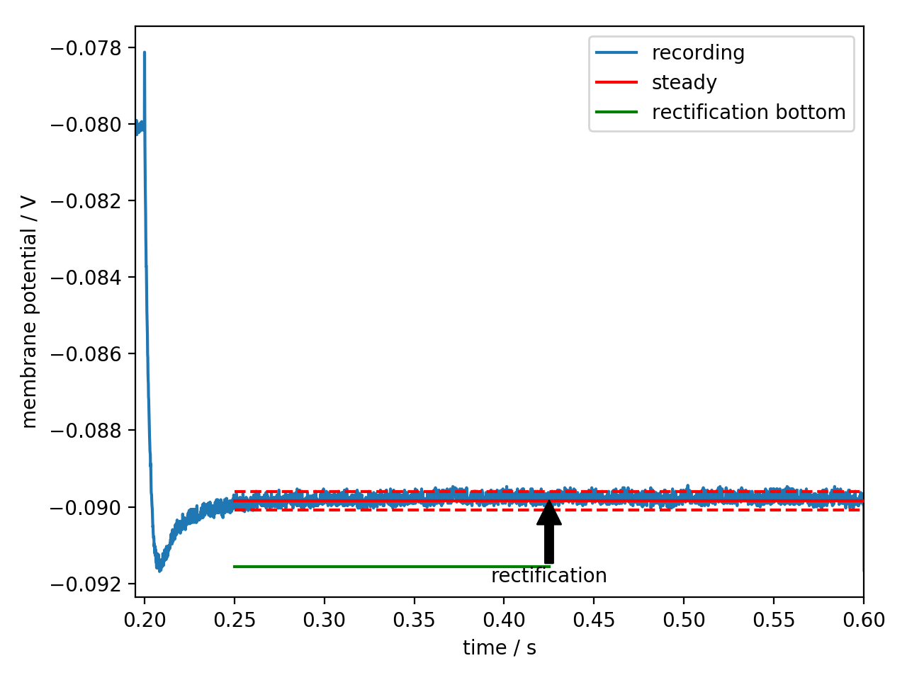
Rectification¶

class ajustador.features.Rectification(obj)[source]¶

(Source code, png, hires.png, pdf)

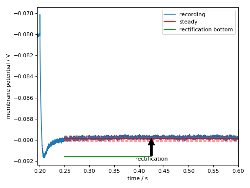
>>> rec = measurements1.waves042811[1]
>>> feat = ajustador.features.Rectification(rec)
>>> print(feat.report())
rectification = 0.0017±0.0001

Additional plots for Rectification

requires = ('injection_start', 'steady_after', 'steady_before', 'falling_curve', 'steady')¶

provides = ('rectification',)¶

array_attributes = ('rectification',)¶

mean_attributes = ('rectification',)¶

window_len = 11¶

rectification¶

plot(figure=None)[source]¶

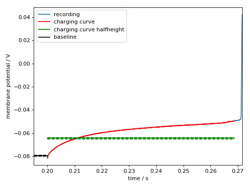
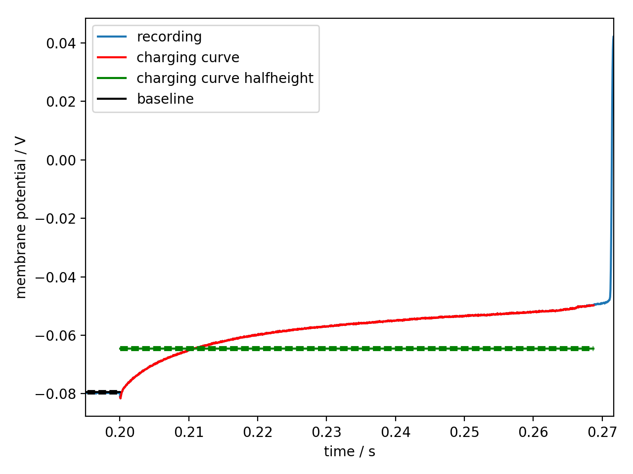
ChargingCurve¶

class ajustador.features.ChargingCurve(obj)[source]¶

(Source code, png, hires.png, pdf)

>>> rec = measurements1.waves042811[-1]
>>> feat = ajustador.features.ChargingCurve(rec)
>>> print(feat.report())
charging_curve_halfheight = 0.01487±0.00002

Additional plots for ChargingCurve

requires = ('wave', 'injection_start', 'baseline', 'baseline_before', 'spikes', 'spike_count', 'spike_threshold')¶

provides = ('charging_curve_halfheight',)¶

array_attributes = ('charging_curve_halfheight',)¶

charging_curve_halfheight¶: The height in the middle between depolarization start and first spike

charging_curve¶

plot(figure=None)[source]¶

ajustador.features¶

SteadyState¶

Spikes¶

AHP¶

FallingCurve¶

Rectification¶

ChargingCurve¶

Table Of Contents

Related Topics

This Page